About sbpy
What is sbpy?
sbpy is an astropy affiliated package for small-body planetary
astronomy. It is meant to supplement functionality provided by
astropy with functions and methods that are frequently used in the
context of planetary astronomy with a clear focus on asteroids and
comets.
As such, sbpy is open source and freely available to everyone. The development
of sbpy is funded through NASA Planetary Data Archiving, Restoration, and
Tools (PDART) Grant Numbers 80NSSC18K0987 and 80NSSC22K0143, but contributions
are welcome from everyone!
Why sbpy?
In our interpretation, sbpy means Python for Small Bodies - it’s
the simplest acronym that we came up with that would neither favor
asteroids nor comets. That’s because we equally like both!
sbpy is motivated by the idea to provide a basis of well-tested and
well-documented methods to planetary astronomers in order to boost
productivity and reproducibility. Python has been chosen as the
language of choice as it is highly popular especially among
early-career researchers and it enables the integration of sbpy into
the astropy ecosystem.
What is implemented in sbpy?
sbpy will provide the following functionality once the development
has been completed:
observation planning tools tailored to moving objects
photometry models for resolved and unresolved observations
wrappers and tools for astrometry and orbit fitting
spectroscopy analysis tools and models for reflected solar light and emission from gas
cometary gas and dust coma simulation and analysis tools
asteroid thermal models for flux estimation and size/albedo estimation
image enhancement tools for comet comae and PSF subtraction tools
lightcurve and shape analysis tools
access tools for various databases for orbital and physical data, as well as ephemerides services
The development is expected to be completed in 2024. For an overview of the progress of development, please have a look at the Status Page.
Additional functionality may be implemented. If you are interested in
contributing to sbpy, please have a look at the contribution guidelines.
Module Structure
sbpy consists of a number of sub-modules, each of which provides
functionality that is tailored to individual aspects asteroid and
comet research. The general module design is shown in the following
sketch.
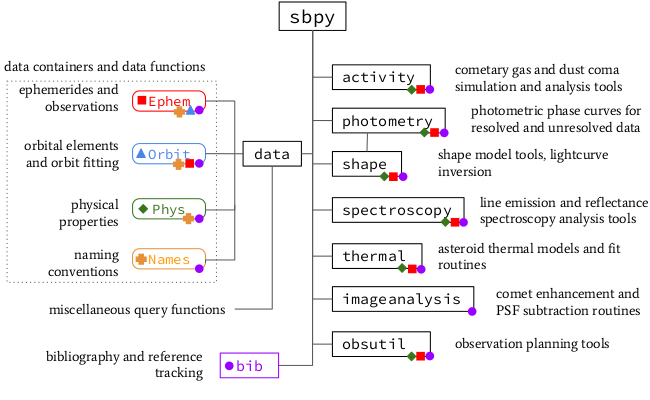
sbpy design schematic. Modules are shown as rectangular boxes,
important classes as rounded colored boxes. The left-hand side of
the schematic is mainly populated with support modules that act as
data containers and query functions. The right-hand side of the
schematic shows modules that focus on small body-related
functionality. Colored symbols match the colors and symbols of
classes and modules they are using.
The functionality of version 1.0, which will be finalized in 2024, is detailed below. Please refer to the Status Page to inquire the current status of each module.
sbpy.data
The data module provides data containers used throughout
sbpy for orbital elements (Orbit), ephemerides
(Ephem), observations (Obs), physical
properties (Phys), and target names
(Names). Instances of these classes are used as input to and
output for a wide range of top-level functions throughout sbpy,
guaranteeing a consistent and user-friendly API. All classes in
data provide query functions to obtain relevant information
from web-based services such as JPL Horizons, Minor Planet
Center (MPC), IMCCE, and Lowell Observatory, providing orbital
elements at different epochs, ephemerides, physical properties,
observations reported to the MPC, (alternative) target identifiers
etc.
Additional functionality of data includes an interface to the
orbit fitting software OpenOrb and an interface to SPICE for offline
ephemerides calculations using SpiceyPy, for which we will provide
utilities tailored to the needs of the small body community. Examples for how to use sbpy with ephemerides calculation package PyEphem and orbital integrator REBOUND (Rein and Liu 2012) will be provided as notebooks.
data also provides a range of other useful module-level
functions: image_search
queries the Solar System Object Image Search function of the
Canadian Astronomy Data Centre, providing a table of images that
may contain the target based on its ephemerides. sb_search uses
IMCCE’s Skybot; given a registered FITS image, the function will
search for small bodies that might be present in the image based on
their ephemerides. pds_ferret queries the Small Bodies Data
Ferret at the Planetary Data Systems Small Bodies Node for all
existing information on a specific small body in the PDS.
sbpy.activity
The activity module provides classes for modeling cometary comae, tails, ice sublimation. We have implemented the Haser gas coma model (Haser, Haser 1957), and a Vectorial model is planned (Vectorial, Festou 1981). Some parameters for commonly observed molecules (e.g., H2O, CO2, CO, OH, CN, C2), such as photo-dissociation timescale and fluorescence band strength, are included. The gas coma classes can be used to generate aperture photometry or a synthetic image of the comet.
For dust, we have simple photometric models based on the Afρ and εfρ quantities (A’Hearn et al. 1984; Kelley et al. 2013). A syndyne/synchrone model (Syndynes, Finson & Probstein 1968; Kelley et al. 2013) is planned.
The activity module includes LTE and non-LTE radiative transfer models used to determine production rates and excitation parameters, such as the temperature in the coma. In the inner regions of the coma collisions dominate molecular excitation and the resulting rotational level population is close to LTE. Beyond the LTE inner region, the level populations start to depart from the equilibrium distribution because the gas density is not high enough to reach thermodynamic equilibrium through collisions with neutrals. The inclusion of all relevant excitation processes in cometary atmospheres in a complex 3-dimensional outgassing geometry represents a state-of-the-art coma model which will provide a baseline for interpretation of cometary spectroscopy observations.
The Cowan & A’Hearn (1979) ice sublimation model (sublimation), used to describe comet activity, and common parameters will also be added.
sbpy.photometry
The photometry module implements a number of light scattering
models for asteroidal surfaces and cometary coma dust. The goal of
this module is to provide a facility to fit light scattering models to
observed brightness data of asteroids, and to estimate the brightness
of asteroids and cometary comae under specified geometry based on
scattering models. Specifically, we include a number of
disk-integrated phase function models for asteroids, bidirectional
reflectance (I/F) models of particulate surfaces, and phase functions
of dust grains in cometary comae. The disk-integrated phase function
models of asteroids include the IAU adopted (H, G1 , G2) system
(Muinonen et al. 2010), the simplified (H, G12) system (Muinonen et
al. 2010) and the revised (H, G12) system (Penttila et al. 2016), as
well as the classic IAU (H, G) system. The
disk-resolved bidirectional reflectance model includes a number of
models that have been widely used in the small bodies community, such
as the Lommel-Seeliger model, Lambert model, Lunar-Lambert model,
etc. Surface facet geometries used in the different models can be
derived with methods in shape. We also include the most
commonly used 5-parameter version of the Hapke scattering
model. Empirical cometary dust phase functions are implemented, too
(Marcus 2007; Schleicher & Bair 2011,
https://asteroid.lowell.edu/comet/dustphase.html). Some
single-scattering phase functions such as the Henyey-Greenstein
function will also be implemented.
sbpy.shape
The shape module provides tools for the use of 3D shape models
of small bodies and the analysis of lightcurve observations. The user
can load asteroid shapes saved in a number of common formats, such as
VRML, OBJ, into Kaasalainen, and then calculate the geometry
of illumination and view for its surface facets, and manipulate
it. Furthermore, Kaasalainen will provide methods for
lightcurve inversion. shape will provide an interface to use
shape models for functions in photometry.
In addition to the shape model methods, shape also provides
methods for the analysis and simulation of simple lightcurve data. The
Lightcurve class provides routines to fit rotational period
(based on Lomb-Scargle routines implemented in stats and other
frequency tools), Fourier coefficients, and spin pole axis
orientation. The class will also be able to simulate a lightcurve at
specified epochs with a shape model class and the associated
information such as pole orientation, illumination and viewing
geometry as provided by the Phys class, and a scattering model
provided through classes defined in the photometry module.
sbpy.spectroscopy
As part of spectroscopy, we provide routines for fitting
measured spectra, as well as simulating synthetic spectra over a wide
range of the electromagnetic spectrum. The spectral models include
emission lines relevant to observations of comet comae, as well as
reflectance spectra of asteroid and comet surfaces. The module
provides functions to fit and remove baselines or slopes, as well as
to fit emission lines or reflectance spectra.
In addition to the aforementioned functionality, we provide a class
Hapke that implements Hapke spectral mixing
functionality.
This module also provides spectrophotometry methods as part of Spectrophotometry. This functionality includes the transmission of spectra (empirical, generated, or from the literature) through common photometric filters, and the derivation of photometric colors from spectral slopes with SpectralGradient.
sbpy.thermal
Thermal modeling capabilities for asteroids are available through the
thermal module. The module provides implementations of the
Standard Thermal Model (STM, Morrison & Lebofsky
1979), the Fast-Rotating Model (FRM, Lebofsky &
Spencer 1989), and the popular Near-Earth Asteroid Thermal Model
(NEATM, Harris 1998) which can all be used in the same
way for estimating fluxes or fitting model solutions to observational
data.
sbpy.imageanalysis
The imageanalysis module will focus on the analysis of
telescopic images. Centroid provides a range of
centroiding methods, including a dedicated comet centroiding technique
that mitigates coma and tail biases (Tholen & Chesley 2004). Code
will also be developed to incorporate ephemerides into FITS image
headers to facilitate image reprojection in the rest frame of the
moving target (moving_wcs) for image co-addition,
e.g., using SWARP (Bertin 2002). We will modify and integrate cometary
coma enhancement code from collaborator Samarasinha
(CometaryEnhancements; Samarasinha & Larson 2014;
Martin et al. 2015). The coma enhancements will be coded into a plugin
for the Ginga Image Viewer.
imageanalysis will also provide PSF subtraction functionality
that is utilizing and extending the Astropy affiliated package
photutils; this class will provide wrappers for photutils to
simplify the application for moving object observations. Results of
imageanalysis.PSFSubtraction routines can be directly used in
imageanalysis.Cometary- Enhancements for further analysis.
sbpy.obsutil
The obsutil module enables the user to conveniently check
observability of moving targets and to plan future observations. Using
Ephem functionality, obsutil provides tools to
identify peak observability over a range of time based on different
criteria, create observing scripts, plot quantities like airmass as a
function of time, and create finder charts for an individual
target. These functions and plots will be easily customizable and will
work identically for individual targets and large numbers of
targets. Finder charts will be produced from online sky survey data,
providing information on the target’s track across the sky, it’s
positional uncertainty, background stars with known magnitudes for
calibration purposes, and other moving objects.
sbpy.bib
bib provides an innovative feature that simplifies the
acknowledgment of methods and code utilized by the user. After
activating the bibliography tracker in bib, references and
citations of all functions used by the user are tracked in the
background. The user can request a list of references that should be
cited based on sbpy functionality that was used at any time as clear
text or in the LATeX BibTex format.
sbpy.calib
sbpy.calib includes calibration methods, including the photometric
calibration of various broad-band filters relative to the Sun’s or
Vega’s spectrum.
Design Principles - The Zen of sbpy
In the design of sbpy, a few decisions have been made to provide a
highly flexible but still easy-to-use API. These decisions are
summarized in the Design Principles, or, the Zen of sbpy.
Some of these decisions affect the user directly and might be considered unnecessarily complicated by some. Here, we review and discuss some of these principles for the interested user.
Physical parameters are quantities
sbpy requires every parameter with a physical dimension (e.g.,
length, mass, velocity, etc.) to be a astropy.units.Quantity
object. Only dimensionless parameters (e.g., eccentricity, infrared beaming
parameter, etc.) are allowed to be dimensionless data types such as floats.
The reason for this decision is simple: every astropy.units.Quantity
object comes with a physical unit. Consider the following example: we
define a Phys object with a diameter for asteroid Ceres:
>>> from sbpy.data import Phys
>>> ceres = Phys.from_dict({'targetname': 'Ceres',
...                         'diameter': 945})
Traceback (most recent call last):
  ...
sbpy.data.core.FieldError: Field diameter is not an instance of <class 'astropy.units.quantity.Quantity'>
Phys.from_dict raised an exception (FieldError) on ‘diameter’ because it was
not an astropy.units.Quantity object, i.e., it did not have units of length.
Of course, we know that Ceres’ diameter is 945 km, but it was not clear from our
definition. Any functionality in sbpy would have to presume that diameters
are always given in km. This makes sense for large objects - but what about
meter-sized objects like near-Earth asteroids?
Following the Zen of Python (explicit is better than implicit), we require that units are explicitly defined:
>>> import astropy.units as u
>>> ceres = Phys.from_dict({'targetname': 'Ceres',
...                         'diameter': 945*u.km})
>>> ceres
<QTable length=1>
targetname diameter
              km
   str5    float64
---------- --------
     Ceres    945.0
This way, units and dimensions are always available where they make sense and we can easily convert between different units:
>>> print(ceres['diameter'].to('m'))
[945000.] m
Epochs must be Time objects
The same point in time can be described by a human-readable ISO time
string ('2019-08-08 17:11:19.196') or a Julian Date
(2458704.216194403), as well as other formats. Furthermore, these
time formats return different results for different time scales: UT
ISO time '2019-08-08 17:11:19.196' converts to '2019-08-08
17:12:28.379' using the TDB time scale.
In order to minimize confusion introduced by different time formats
and time scales, sbpy requires that epochs and points in time are
defined as Time objects, which resolve this confusion:
>>> from sbpy.data import Obs
>>> from astropy.time import Time
>>> obs = Obs.from_dict({'epoch': Time(['2018-01-12', '2018-01-13']),
...                      'mag': [12.3, 12.6]*u.mag})
>>> obs['epoch']
<Time object: scale='utc' format='iso' value=['2018-01-12 00:00:00.000' '2018-01-13 00:00:00.000']>
Time objects can be readily converted into other formats:
>>> obs['epoch'].jd
array([2458130.5, 2458131.5])
>>> obs['epoch'].mjd
array([58130., 58131.])
>>> obs['epoch'].decimalyear
array([2018.03013699, 2018.03287671])
>>> obs['epoch'].iso
array(['2018-01-12 00:00:00.000', '2018-01-13 00:00:00.000'], dtype='<U23')
as well as other time scales:
>>> obs['epoch'].utc.iso
array(['2018-01-12 00:00:00.000', '2018-01-13 00:00:00.000'], dtype='<U23')
>>> obs['epoch'].tdb.iso
array(['2018-01-12 00:01:09.184', '2018-01-13 00:01:09.184'], dtype='<U23')
>>> obs['epoch'].tai.iso
array(['2018-01-12 00:00:37.000', '2018-01-13 00:00:37.000'], dtype='<U23')
See Epochs and the use of astropy.time and Time for additional information.
Use sbpy DataClass objects
Finally, we require that topically similar parameters are bundled in
DataClass objects, which serve as data containers (see
this page for an introduction).
This containerization makes it possible to keep data neatly formatted and to minimize the number of input parameters for functions and methods.